Establishing Dilution Linearity for Your Samples in an ELISA
The purpose of dilution linearity experiments
When testing a new Host Cell Protein (HCP) immunoassay, establishing dilution linearity is a foundational experiment to help you determine if the chosen HCP ELISA is appropriate for the population of HCPs in your in-process and Drug Substance samples. When performed correctly, dilution linearity will inform experimental conditions needed for further assay qualification studies, so it is the first assay you should perform.
Specifically, dilution linearity experiments serve to establish the dose-response curve and full quantitative range of the assay for your process HCPs. When dilution linearity is successfully demonstrated for a given sample type, it confirms that the important condition of antibody excess is met for the diverse array of HCPs present in your samples, and that the sample matrix does not hinder HCP quantification, allowing you to have confidence in your results.
How to approach dilution linearity experiments
Any sample type with suspected levels of contaminants greater than the limit of quantification (LOQ) of the assay should initially be evaluated for dilution linearity. This experiment involves performing several serial dilutions using an approved assay diluent. These dilutions are then assayed, and a dilution-corrected HCP concentration is determined at each dilution. In most cases, a dilution will be reached where the dilution-corrected value remains relatively constant with minimal variation. This dilution is referred to as the Minimum Required Dilution (MRD).
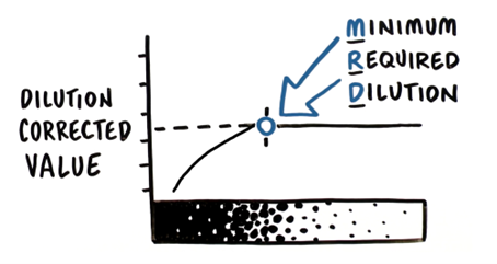
In this example (Table 1), the sample did not demonstrate good dilution linearity at high concentrations (neat, 1:2 and 1:4), but with further dilution, an MRD was determined at which acceptable dilution linearity is achieved. By definition, acceptable dilution linearity is reached when corrected analyte concentrations vary no more than ±20% between doubling dilutions, avoiding the lower end of the assay range where the assay value before correction falls below two times the assay LOQ (in this example, 1:64). The percent change can be calculated by subtracting the previous dilution-corrected value and then dividing the difference by the corrected value for that dilution. For example, a percent change of 60% is determined for the 1:2 dilution by the following equation: [(233-146)/146] x 100%.
Sample Dilution | Dilution Corrected Value (ng/mL) | % Change in concentration from previous dilution |
Neat (undiluted) | 146 | NA |
1:2 | 233 | 60% |
1:4 | 312 | 34% |
1:8 | 361 | 16% |
1:16 | 356 | 1% |
1:32 | 370 | 4% |
1:64 | Not calculated (<2 times LOQ) | NA |
Table 1. Sample Dilution Linearity Data.
From this data, we conclude that the MRD for this in-process sample is 1:4 and report the HCP concentration as the average of the results at/below the MRD and above the LLOQ (in this case, the average of 312, 361, 356, and 370 is reported as 350 ng/mL).
Ideally, dilution linearity evaluation should be performed for any type of sample you will routinely test, including in-process samples as well as your final drug substance. Once the MRD is established for each sample type and matrix, you should include specific guidance on how to dilute each sample in your SOP.
Troubleshooting poor dilution linearity
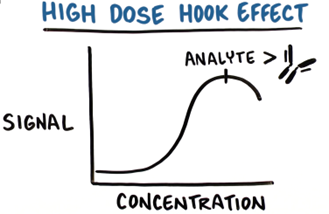
For assays that detect more than one type of analyte, such as HCP ELISAs, a lack of dilution linearity may be observed for certain samples and concentrations. In such cases, this typically means that antibody excess is not met for one or more types of analyte present in the sample. For example, very high concentrations of certain HCPs may elicit a “high-dose hook effect” by saturating the antibody against that particular HCP, which will result in under-quantitation of that HCP.
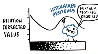
Additionally, certain hitchhiker proteins may interact with your product and/or become significantly enriched during the purification process, and thus interfere with the linearity of the assay altogether.
Other causes for poor dilution linearity are due to certain components in product formulation buffer interfering with the ability of the assay to detect HCPs or other contaminants, resulting in over- or under-estimation of the true HCP concentration.
Remember: it is only under conditions of antibody excess that the dose response curve is positively sloped and the assay quantitation accurate.
If the antibody is in a limiting concentration or if the sample matrix causes a negative interference, you will observe that the apparent HCP concentration for a given sample increases as it is further diluted, necessitating further dilution of the sample. In other cases, modification of the assay protocol can improve accuracy for some sample types. If additional dilution of the sample does not resolve the poor dilution linearity, there could be a problem with the purification process. Users of our kits are encouraged to contact our Technical Services Department for advice on how best to solve dilution linearity issues.
Next steps
Once you have successfully achieved dilution linearity for your samples, additional spike and recovery as well as precision experiments should be performed to ensure your assay is fit-for-purpose. Watch our video and check out our spike and recovery post to learn more about these critical experiments: